What is a Pandas DataFrame?
I’m reading Jake VanderPlas’s “Python Data Science Handbook”. I’ve been using the Python data analysis library Pandas for a while, but I sometimes feel clumsy and confused at its apparent quirks. It has helped to go back to basics and review what a DataFrame is, along with Series and Indexes.
Disclaimer: This post sketches out how a DataFrame can be thought of. The actual implementation doesn’t exactly match!
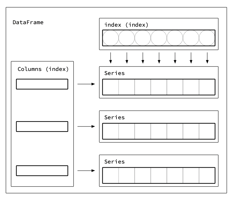
DataFrames are a dictionary mapping column names to Series
The documentation says a DataFrames
“Can be thought of as a dict-like container for Series objects.”
Let’s start with a “proto-DataFrame” as a dictionary mapping a column name to a pd.Series. For now, a Series can be thought of as a list of values.
Let’s take a sample dataset. Say we have an aggregated dataset of how many books are checked out at different branches of a library on a minute-level.
checkout_time,        ballard_count,   downtown_count
2016-07-30 11:24:00               1,               10
2016-07-30 11:25:00               2,                0
2016-07-30 11:26:00               0,                2
2016-07-30 11:28:00               2,                0
2016-07-30 11:29:00               2,                0
2016-07-30 11:30:00               1,                4
A DataFrame would create a Series for each column. For example, the ballard_count
could be a Series like:
ballard_counts_series = pd.Series([
  1,
  2,
  0,
  2,
  2,
  1,
])
Then the proto-DataFrame could work like this:
checkouts_fake_df = {
    'checkout_time': checkout_series,
    'ballard_count': ballard_counts_series,
    'downtown_count': downtown_counts_series,
}
The following image illustrates the information above.

The proto-DataFrame structure gives us a feature that Pandas DataFrames have: we can access a column using the column name:
>> checkouts_fake_df['ballard_count']
[ 1, 2, 0, 2, 2, 1 ]
However, in Pandas, we can also request “rows 3 through 5” as if a DataFrame was a list of rows!
>> checkouts_df[3:5]
2016-07-30 11:28:00   1   0
2016-07-30 11:29:00   2   0
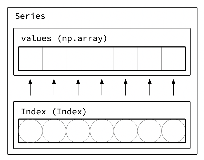
Our proto-DataFrame can’t support indexing by slices. Real DataFrames do this with the help of “Indexes.” To describe them, let’s first look at a Series data structure.
Series
Series are typically a 1D numpy array with some additional information including the dtype and an index.
Series data
Pandas typically stores a Series’ values as a numpy array. Numpy and Pandas have implementations of many efficient operations for numpy arrays. For example, there are fast element-wise addition and substring operations. Even more functions can be found on the universal functions (ufuncs) page).
Series dtype
I was curious why a DataFrame mapped column names to Series, instead of mapping row labels to row data. This choice makes more sense when thinking about how arrays usually work. One reason numpy arrays are efficient is that if we assume each element of an array has the same size, we can store the data next to each other in memory and just point to the right location. VanderPlas gives a nice description of what Python is doing under the hood. As an abridged summary, a normal Python list might use a linked list and store datatype information for every item in a list. In a Numpy array of integers, the data is stored with a single copy of the datatype and the data as an array.
For intuition, compare how much text there is in the “list of ints”
[
  {type: np.int64, value: 0},
  {type: np.int64, value: 1},
  {type: np.int64, value: 2},
  {type: np.int64, value: 3},
  {type: np.int64, value: 4},
]
compared to a “integer array”
{
  type: np.int64,
  value: [
    0,
    1,
    2,
    3,
    4,
  ]
}
Being able to store data efficiently is one of the reasons why DataFrames start as a dictionary of Series instead of a list of rows! It also has a lot of parallels with Column-oriented databases
dtype for a Series with multiple data types
That said, sometimes we do need a column with multiple data types. Pandas allows multiple datatypes in a column while still obeying the “everything in this array is the same type” by making every item into a pointer to the object. However, using objects causes a decrease in performance, especially for large arrays.
Series: Index
Now that we have the basics of a Series, let’s revisit how to be able to access a slice of rows. To do this, a Series also has an Index to make it convenient to look up items.
Returning to the library checkout example, I’ll create a Series for the downtown_counts_series data. There’s only one row per checkout time, so I’ll set the index to the time the books were checked out.
index = pd.to_datetime([
  '07/30/2016 11:23:00 AM',
  '07/30/2016 11:24:00 AM',
  '07/30/2016 11:25:00 AM',
  '07/30/2016 11:26:00 AM',
  '07/30/2016 11:27:00 AM',
  '07/30/2016 11:29:00 AM',
  '07/30/2016 11:30:00 AM',
])

values = [1, 2, 1, 2, 2, 1, 1]

downtown_counts_series = pd.Series(data=values, index=index)
The above code creates a Series like this:
2016-07-30 11:23:00    1
2016-07-30 11:24:00    2
2016-07-30 11:25:00    1
2016-07-30 11:26:00    2
2016-07-30 11:27:00    2
2016-07-30 11:29:00    1
2016-07-30 11:30:00    1
dtype: int64
As expected, we can look up the value for a given time.
> time_index = pd.to_datetime('2016-07-30 11:28:00')
> ballard_counts_series[time_index]
In addition, we can select a range of times. For example, to select the times between 11:25 and 11:30, we can use:
>> ballard_counts_series['2016-07-30 11:28:00':'2016-07-30 11:30:00']
2016-07-30 11:28:00    2
2016-07-30 11:29:00    2
2016-07-30 11:30:00    1
dtype: int64
Element-wise functions align along indexes!
Let’s say we want to add downtown_counts_series to a new ballard_counts_series in order to find the total checkouts between both branches.
However, not all libraries had values for every minute.
index = pd.to_datetime([
  '07/30/2016 11:23:00 AM',
  '07/30/2016 11:25:00 AM',
  '07/30/2016 11:28:00 AM',
  '07/30/2016 11:30:00 AM',
])


values = [10, 2, 4, 2]

ballard_counts_series = pd.Series(data=values, index=index)

ballard_counts_series + downtown_counts_series
Adding the two series aligns the indexes. In this case, the null values also propogate.
(Also you’ll notice that when NaN is introduced, integers turn into floats! This is because the default missing value in Pandas, np.nan, is a float. Because Pandas tries to make arrays that have the same type, ints get turned into floats!)
2016-07-30 11:24:00    11.0
2016-07-30 11:25:00     NaN
2016-07-30 11:26:00     NaN
2016-07-30 11:28:00     NaN
2016-07-30 11:29:00     NaN
2016-07-30 11:30:00     6.0
dtype: float64

In order to default to 0, we can use the special .add method.
downtown_counts_series.add(ballard_counts_series, fill_value=0)
2016-07-30 11:24:00    11.0
2016-07-30 11:25:00     2.0
2016-07-30 11:26:00     2.0
2016-07-30 11:28:00     1.0
2016-07-30 11:29:00     2.0
2016-07-30 11:30:00     6.0
dtype: float64
Back to DataFrames
Let’s take knowledge about Series back to DataFrames! When DataFrame has multiple Series, the union of the indexes are shared across all Series.
For example, we can create a DataFrame with the two Series from before.
pd.DataFrame({
    'ballard_count': ballard_counts_series,
    'downtown_count': downtown_counts_series,
})
As with operations, creating a DataFrame aligns the indexes and fills missing values with NaN.
                       ballard_count    downtown_count
2016-07-30 11:23:00              1.0               0.0
2016-07-30 11:24:00              1.0              10.0
2016-07-30 11:25:00              2.0               NaN
2016-07-30 11:26:00              NaN               2.0
2016-07-30 11:28:00              2.0               NaN
2016-07-30 11:29:00              2.0               NaN
2016-07-30 11:30:00              1.0               4.0
We can also adjust the DataFrame index, which will adjust both Series. In this example, 11:27:00 is missing.
We can fill the missing values with zero, and then convert the data back to integers.
lib_df.resample('T').asfreq().fillna(0).astype('int')
                       ballard_count    downtown_count
2016-07-30 11:23:00                1                 0
2016-07-30 11:24:00                1                10
2016-07-30 11:25:00                2                 0
2016-07-30 11:26:00                0                 2
2016-07-30 11:27:00                0                 2
2016-07-30 11:28:00                2                 0
2016-07-30 11:29:00                2                 0
2016-07-30 11:30:00                1                 4
Summary and see also
A DataFrame is made up of three key components: the data, an Index of columns, and an Index of rows. The data can be thought of as a Series for each column. The data in a column tends to have the same type, which allows for efficient storage and manipulation. A ton of Panda’s complexity and power comes from the Index, including selecting time ranges and aligning data before doing operations.
I think starting to understand DataFrames helps me make sense of Pandas’ quirks.
See Also
- For more Pandas tips, check out Jake VanderPlas’s Python Data Science Handbook
- Pandas documentation