Neural style transfer
The last few weekends, I’ve been experimenting with neural style transfer. Style transfer combines two images to create a new image with similar content as one image but using the style from the other image.
For example, using the technique in the paper A Neural Algorithm of Artistic Style and code from the example implementation from Keras, I can produce stylized images of Mt. Hood.
| Original | Tsunami | The Scream | Primordal Chaos |
|---|---|---|---|
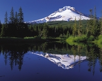 |
 |
 |
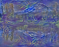 |
 |
 |
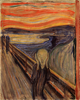 |
 |
This post shows what the technique is doing and includes an implementation heavily based on Keras’s example implementation.
After some nice examples of how it should work in theory, I also note some learnings and weird results.
Source images
This technique combines two images: a content image and a style image.
(As usual, the full notebook is on github.)
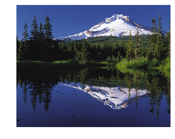
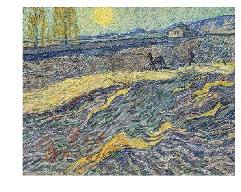
Start with a pretrained network
Often in deep learning, you need to train a network on a lot of data to get good results. However, this neural style transfer technique starts with a network that has already been trained on huge amounts of data.
I used the VGG19 packaged with Keras which has been trained on the gigantic ImageNet dataset. VGG19 on ImageNet was trained to classify what was in images (e.g. tell that a picture is of a “car”).
from keras.applications import vgg19

regular_vgg = vgg19.VGG19(weights='imagenet', include_top=False)

regular_vgg.summary()
_________________________________________________________________
Layer (type) Output Shape Param #
=================================================================
input_1 (InputLayer) (None, None, None, 3) 0
_________________________________________________________________
block1_conv1 (Conv2D) (None, None, None, 64) 1792
_________________________________________________________________
block1_conv2 (Conv2D) (None, None, None, 64) 36928
_________________________________________________________________
block1_pool (MaxPooling2D) (None, None, None, 64) 0
_________________________________________________________________
block2_conv1 (Conv2D) (None, None, None, 128) 73856
_________________________________________________________________
block2_conv2 (Conv2D) (None, None, None, 128) 147584
_________________________________________________________________
block2_pool (MaxPooling2D) (None, None, None, 128) 0
_________________________________________________________________
block3_conv1 (Conv2D) (None, None, None, 256) 295168
_________________________________________________________________
block3_conv2 (Conv2D) (None, None, None, 256) 590080
_________________________________________________________________
block3_conv3 (Conv2D) (None, None, None, 256) 590080
_________________________________________________________________
block3_conv4 (Conv2D) (None, None, None, 256) 590080
_________________________________________________________________
block3_pool (MaxPooling2D) (None, None, None, 256) 0
_________________________________________________________________
block4_conv1 (Conv2D) (None, None, None, 512) 1180160
_________________________________________________________________
block4_conv2 (Conv2D) (None, None, None, 512) 2359808
_________________________________________________________________
block4_conv3 (Conv2D) (None, None, None, 512) 2359808
_________________________________________________________________
block4_conv4 (Conv2D) (None, None, None, 512) 2359808
_________________________________________________________________
block4_pool (MaxPooling2D) (None, None, None, 512) 0
_________________________________________________________________
block5_conv1 (Conv2D) (None, None, None, 512) 2359808
_________________________________________________________________
block5_conv2 (Conv2D) (None, None, None, 512) 2359808
_________________________________________________________________
block5_conv3 (Conv2D) (None, None, None, 512) 2359808
_________________________________________________________________
block5_conv4 (Conv2D) (None, None, None, 512) 2359808
_________________________________________________________________
block5_pool (MaxPooling2D) (None, None, None, 512) 0
=================================================================
Total params: 20,024,384
Trainable params: 20,024,384
Non-trainable params: 0
_________________________________________________________________
VGG19 examples
A hand-wavy explanation of why this is useful is that the trained VGG19 network has already learned a good way to represent images. For example, to identify “a car”, maybe the network learned that a car has shiny surfaces (and superficial features like “shiny” are in theory detected by lower-valued blocks of the network) and that a car has four wheels and is usually on a road (and more abstract features, such as neurons for “wheel” and ones for “road”, are in higher-valued blocks of the network). The neural style transfer technique I’m using works by trying to draw the abstract features from the content image, such as “wheels” and “road”, while matching the superficial features from the style image, such as “shiny” or “lots of blue brush strokes”.
To get an idea of those “wheel” neurons, we can look at what VGG19 produces at different layers.
def create_vgg_layer_outputs(input_tensor):
    vgg = vgg19.VGG19(input_tensor=input_tensor, weights='imagenet', include_top=False)

    # order all of the outputs and their names
    vgg_layer_outputs = [
        (layer.name, layer.output)
        for layer in vgg.layers
    ]
    layer_names, layer_outputs = zip(*vgg_layer_outputs)

    # evaluate the outputs all at once
    output_values = K.function([], layer_outputs)([])

    # and return the labeled output values
    return dict(zip(layer_names, output_values))
Content image convolutional outputs
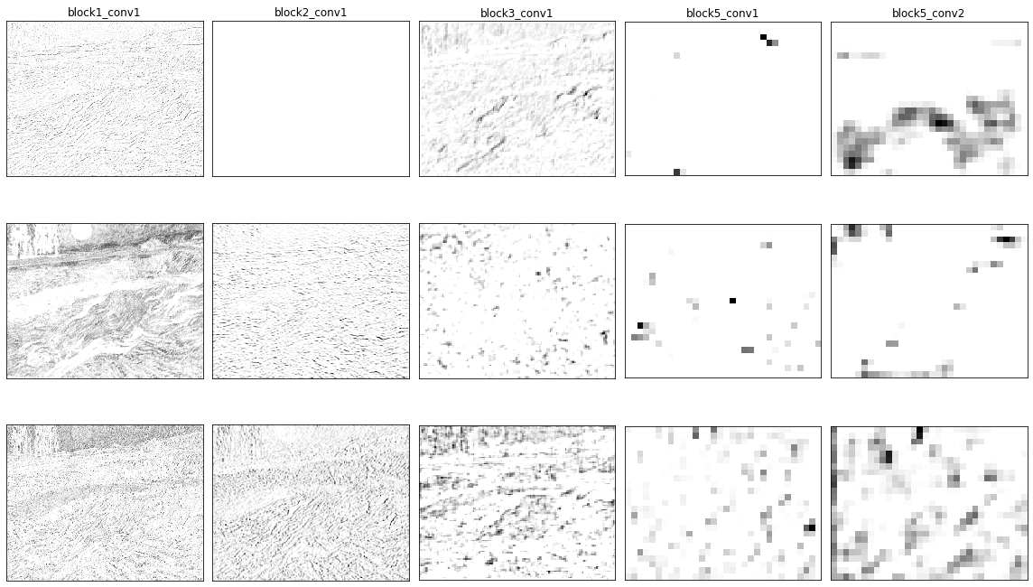
Let’s look inside and see how the network represents the content image. I’ll go to various layers and print out what a few features look like.
I’m only printing 3 filters from each layer (for example, block5_conv1 has 512 filters), so this is just a peek into how the network is representing the image.

Style image convolutional outputs
For fun, I can do the same on the style image.
Setting up a loss function
In order to make an image that combines the images, I’ll have the network nudge the pixel values of a third image, which I call the “variable image.” To guide how to nudge the image, the paper describes a loss function based on a “content loss” and a “style loss”. The Keras code adds a “variational loss.”
Content loss
The content loss tries to get a deep layer, such as block5_conv2, of the content image to match the variable image. Since the deep layers should represent larger, abstract items (“a tower”, “some grass”, “the sky”), the content loss should encourage the resulting image to share the content of the image.
Style loss
The style loss tries to get shallower layers, such as block1_conv1, from the style image to match the variable image.
Instead of matching the layers values directly, the style loss is based on the Grams matrix of vectorized features layer. That means that all information about the location is squashed.
(Aside: I wrote a little another use of Grams matrix here).
Variational loss
The variational loss penalizes the variable image if pixels next to each other are very different. This smooths the resulting image.
Defining which layers to use
Typically, “shallow layers” should have a non-zero style weight, and “deeper layers” should have a non-zero content weight. I set my implementation up so I could configure which layers to use and how much to weight each layer.
from collections import namedtuple

LayerWeights = namedtuple('LayerWeights', ['layer_name', 'style_weight', 'content_weight'])

layer_weights = [
    LayerWeights('block1_conv1', style_weight=1, content_weight=0.0),
    LayerWeights('block2_conv1', style_weight=1, content_weight=0.0),
    LayerWeights('block3_conv1', style_weight=1, content_weight=0.0),
    LayerWeights('block4_conv1', style_weight=1, content_weight=0.0),
    LayerWeights('block5_conv1', style_weight=1, content_weight=0.0),
    LayerWeights('block5_conv2', style_weight=0.0, content_weight=1e2),
]
Now I’ll define a loss_from_layer_weights based on the provided layer_weights.
# Borrowing a few more functions from the Keras example
def sum_squared(content, variable):
    return K.sum(K.square(content - variable))

# This returns a matrix with the size [3, FEATURE_SIZE, FEATURE_SIZE]
def gram_matrix(x):
    features = K.batch_flatten(K.permute_dimensions(x, (2, 0, 1)))
    gram = K.dot(features, K.transpose(features))
    return gram
def loss_from_layer_weights(layer_weights, vgg_layer_outputs, variable_tensor):
loss = K.variable(0.0)
for layer in layer_weights:
# Separate the three images again
content_layer_out = vgg_layer_outputs[layer.layer_name][0]
style_layer_out = vgg_layer_outputs[layer.layer_name][1]
variable_layer_out = vgg_layer_outputs[layer.layer_name][2]
# All images should be the same time
width, height, filters = content_layer_out.shape
# Add the content weights
loss += layer.content_weight * sum_squared(content_layer_out, variable_layer_out)
# Add the style weights
# The paper divides the style loss by 4 * M**2 * N**2.
style_denominator = 4 * int(width * height * filters) ** 2
loss += layer.style_weight * sum_squared(
gram_matrix(style_layer_out),
gram_matrix(variable_layer_out)
) / style_denominator
# Add variation loss to make sure pixels next to each other are similar
raw_variation_loss = (
K.square(variable_tensor[:, :-1, :-1] - variable_tensor[:, 1:, :-1])
+ K.square(variable_tensor[:, :-1, :-1] - variable_tensor[:, :-1, 1:])
)
total_variation_loss = K.sum(K.pow(raw_variation_loss, 1.25))
loss += total_variation_loss
return loss def neural_style_loss(
content_tensor,
style_tensor,
variable_tensor,
layer_weights):
input_tensor = K.concatenate([
content_tensor,
style_tensor,
variable_tensor,
], axis=0)
# Get a VGG model
vgg = vgg19.VGG19(input_tensor=input_tensor, weights='imagenet', include_top=False)
# Name all of VGG's layers
vgg_layer_outputs = {
layer.name: layer.output
for layer in vgg.layers
}
# Build the loss function
loss = loss_from_layer_weights(
layer_weights,
vgg_layer_outputs,
variable_tensor,
)
# Return a function that, given the variable tensor, will return the loss and gradients.
grads = K.gradients(loss, variable_tensor)
return K.function([variable_tensor], [loss] + grads)
f_loss_and_grads = neural_style_loss(
content_tensor,
style_tensor,
variable_tensor,
layer_weights
)Initializing the image
My favorite results happened when I initialized with random noise.

Fitting the model
With f_loss_and_grads, I have a function that can tell me how far the variable image is from the ideal image. Now I need a way to update the variable image to make it closer to ideal!
There are a few choices of optimizers. The Keras example uses scipy’s fmin_l_bfgs_b. It needs a function that returns the loss function’s value for an image, and a function that returns and the loss function’s gradients for an image.
(I also used BFGS in my logistic regression post!)
# Again, borrowing from the Keras example. `f_loss_and_grads` takes a few seconds to run.
# Instead of calling it twice, the Keras example stores the results.

class GradientAndLoss():
    def __init__(self):
        self._grad = None
        self._loss = None

    def loss(self, flat_image):
        assert self._grad is None
        self._loss, self._grad = f_loss_and_grads([
            flat_image.reshape((1, *target_image_size))
        ])
        return self._loss

    def grad(self, flat_image):
        assert self._grad is not None
        grad = np.copy(self._grad)
        self._loss = None
        self._grad = None
        return grad.flatten().astype('float64')

gradient_and_loss = GradientAndLoss()
Now I run the following code block on a GPU a few times until I get a good image.
<img width=300px src=”/assets/2019-03-17-result.png”>
Results
Now that I have a better image, I can compare it to the original. I should see that the content layers match the content. I might notice the style image being similar.

Etc
This project was neat. Besides making images I think are cool, it’s an example of a deep learning project that doesn’t need a lot of custom data: I just need the style image and content image and the VGG19 network weights.
Failed images
In this post, I showed some cool images, but many of the combinations I tried resulted in muddy images that didn’t look very good. I think there’s a reason certain images (Starry Night, The Scream, Tsunami, Picasso) are so common in Neural Style Transfer posts! There are a lot of choices in parameters, and the scaling of the image influences the layer detection. It’s hard to tell if combinations would turn out better if I had tweaked the parameters right, or if the method wouldn’t work. For example, in the example below, some parameters weren’t weighted right.
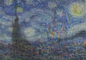
Oh no, the Uppsala cathedral is a ghost. style, content
Also some of my favorite results didn’t really copy the style, but just made a cool looking result (Primordial Chaos, and the Sutro Tower image below).

Code
I really like being able to implement methods from scratch.
So I feel a little weird that this post is mostly the provided Keras example, with different configuration (I like my namedtuples), and some code deleted or moved around.
I started this post by trying to implement Neural Style Transfer in Keras using the paper from scratch. My method was slow and images weren’t turning out very good (looking back, that might be in part because of the technique, and not running on a GPU.) Also a few things in the implementation felt awkward: for example, I was feeding in the same image in each epoch.
GPUs
My laptop was pretty slow at generating the images, so I used a GPU in Colaboratory.
Other posts
- One more time, the provided Keras example