Climate classification with neural networks
The Köppen Climate classification is a widely used climate classification system. It classifies locations around the world as climates like “Tropical rainforest” or “Warm summer continental”.
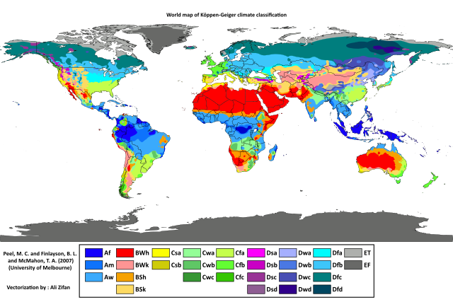
(Image from Wikipedia and [1])
One funny thing about the Köppen classification is that it puts Portland, Oregon in the same group as San Francisco and in a very similar group to Los Angeles. I might be wrong, but Southern California (comfortably walking outside in a t-shirt at 2am) seemed like a pretty different climate than Seattle (not seeing the sun for n months)!
I wanted to try classifying climates of locations. In this post, I’ll try to classify the climate of continental US weather stations based on the weather they recorded with the help of a neural net. I’ll train a neural net on some task that also helps it learn vector representations for each station. Then I’ll cluster the vector representations to cluster similar stations into climate classifications.
Data
I used data from the Global Historical Climatology Network [2, 3]. I used the subset of weather stations from the U.S. Historical Climatology Network.
This gives 2.4G of data containing decades (sometimes over a century!) of daily weather reports from 1,218 stations around the US. It usually gives high temperatures, low temperatures, and precipitation, but also gives information about snow, wind, fog, evaporation rates, volcanic dust, tornados, etc.
Getting the data
Wheee, let’s download a few GBs of historical weather data.
The readme is super useful.
The tar file for the US stations is located at ftp://ftp.ncdc.noaa.gov/pub/data/ghcn/daily/ghcnd_hcn.tar.gz (heads up, it uses an underscore, not a hyphen like the readme says!)
The other useful file is ftp://ftp.ncdc.noaa.gov/pub/data/ghcn/daily/ghcnd-stations.txt, which contains coordinates and station names.
Weather stations
If I go through the .dly files in ghcnd_hcn/ folder, and look up the station names in ghcnd-stations.txt, I can plot the stations I have daily weather records for using Basemap. (See “Basemap” below for code and details.)

Reducing the data
The script I used for processing data is located here.
There are two issues with the dataset: it’s a little large to easily load and manipulate in memory and some records are missing or are labeled as low-quality. I’d love to figure out how to use larger datasets or handle the low-quality data, but I’ll save that for another post. Instead, I’ll create a small subset I can comfortably load into memory. For each station, I’ll sample up to 2000 daily weather reports, including the maximum temperature, minimum temperature, and precipitation.
I limit the data in a few ways. I dropped data before 1990 to make the datasets more manageable. I also require all three weather values are not missing and don’t have a quality issue. These may introduce bias. If I was doing real science instead of trying to make a pretty graph, I’d justify these decisions better!
Loading the dataset
See scripts/process_weather_data.py for details, but if you ran the command in this folder using data/weather/data as the output file, such as:
python scripts/process_weather_data.py [filtered .dly files, see process_weather_data] data/weather/data
then I think this code should work.
DATA_PATH = 'data/weather'
matrix_file = os.path.join(DATA_PATH, 'data/gsn-2000-TMAX-TMIN-PRCP.npz')
# column labels
STATION_ID_COL = 0
MONTH_COL = 1
DAY_COL = 2
VAL_COLS_START = 3
TMAX_COL = 3
TMIN_COL = 4
PRCP_COL = 5
with np.load(matrix_file) as npz_data:
weather_data = npz_data['data'].astype(np.int32)
print(weather_data.shape)
# I decided to switch over to using the day of the year instead of two
# eh, this isn't perfect (it assumes all months have 31 days), but it helps differentiate
# the first of the month vs the last.
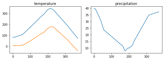
weather_data_day_of_year_data = 31 * (weather_data[:, MONTH_COL] - 1) + (weather_data[:, DAY_COL] - 1)To give an idea of how this data looks, here’s the number of examples per station, the minimum and maximum temperature.
There are a few things I’m overlooking for now: the weather report values are always integers and precipitation is always positive. Precipitation has a larger range and is often 0. I’ll end up converting the month and day into the approximate day of the year (e.g., 21 = January 21), which means January 1 and December 31 are considered far apart.

Neural network
The purpose of the neural network is to learn a good vector representation of the weather station. To do this, I’ll set up a task that hopefully encourages the network to learn a good vector representation.
The inputs are the station_id and day of the year (so the month and day, but the year is missing).
The network needs to predict the precipitation, high temperature and low temperature for that day. I compare its prediction to an arbitrary year’s actual weather and use how poorly it does to tell TensorFlow how to update the network parameters.
To get the vector representation, I pass the station_id through an embedding layer. Then I concatenate the day to make a bigger vector. I’ll pass the station+day vector through a little neural network that needs to predict the three weather values. The full network looks something like this:

In the image above, the weather data from U.S. Historical Climatology Network gives me the blue and green boxes. I’m using the left-most boxes (station_id and day) as input and the right-most boxes (precipitation, high temperature, low temperature) as output. As I train the model, back-propagation will find better parameters for the blue boxes (the station vector representations and the neural network.)
When I’m satisfied, I’ll take the vector representation and use an unsupervised classifier on it I don’t particularly care about the neural network learns. I’m just using it to learn the vector representations. Once I have the vector representations, I’ll use K-Means clustering to cluster stations that have similar vectors. These clusters will become my climate classification!
Defining the network
Below I implement the network in TensorFlow.
tf.reset_default_graph()

# set up the batch and input data
InputBatch = namedtuple('InputBatch', [
    'station_ids',
    'month_day',
])

# let's try out tf.data! set up the dataset and iterator.
with tf.variable_scope('data_loading'):
    station_id_placeholder = tf.placeholder(tf.int32, (None,), name='station_id_placeholder')
    month_day_placeholder = tf.placeholder(tf.float32, (None,), name='month_day_placeholder')  # day of the year
    target_placeholder = tf.placeholder(tf.float32, (None, 3), name='target_placeholder')

    dataset = tf.data.Dataset.from_tensor_slices((
        InputBatch(
            station_ids=station_id_placeholder,
            month_day=month_day_placeholder,
        ),
        target_placeholder # and grab all the weather values
    ))\
    .shuffle(buffer_size=10000)\
    .repeat()\
    .batch(BATCH_SIZE)

    iterator = dataset.make_initializable_iterator()
    input_batch, targets = iterator.get_next()

# Feed the station id through the embedding. This embeddings variable
# is the whole point of this network!
embeddings = tf.Variable(
    tf.random_uniform(
        [NUM_STATIONS, EMBEDDING_SIZE], -1.0, 1.0),
    dtype=tf.float32,
    name='station_embeddings'
)

embedded_stations = tf.nn.embedding_lookup(embeddings, input_batch.station_ids)

# Drop in the month/day data
station_and_day = tf.concat([
    embedded_stations,
    tf.expand_dims(input_batch.month_day, 1),
], axis=1)

# Now build a little network that can learn to predict the weather
dense_layer = tf.contrib.layers.fully_connected(station_and_day, num_outputs=HIDDEN_UNITS)
with tf.variable_scope('prediction'):
    prediction = tf.contrib.layers.fully_connected(
        dense_layer,
        num_outputs=3,
        activation_fn=None, # don't use an activation on prediction
    )

# Set up loss and optimizer
loss_op = tf.losses.mean_squared_error(prediction, targets)
tf.summary.scalar('loss', loss_op)
train_op = tf.train.AdamOptimizer().minimize(loss_op)

# And additional tensorflow fun things
merged_summaries = tf.summary.merge_all()
init = tf.global_variables_initializer()
saver = tf.train.Saver()
Clustering
As the model is training, I’ll occasionally cluster the stations and save the results.
def save_classification(save_location, trained_embeddings):
    kmeans = KMeans(n_clusters=CLUSTER_NUMBER, random_state=0).fit(trained_embeddings)

    with open(save_location, 'w') as f:
        for station, label in zip(stations, kmeans.labels_):
            f.write('{}\t{}\n'.format(station, label))
Now I can start training! You can monitor the job through TensorBoard.
Deciding when to stop
If I had a metric for how good the climate classifications were, I could use the metric to decide when the model is done training. For the purpose of this post (again, pretty pictures), I’ll just train the model long enough to run through the dataset a few times.
(I have 2.4M weather reports. Since I’m using batch size of 50, it will take around 50K steps will go through the dataset once.)
MAX_STEPS = 1000000
CHECKPOINT_EVERY_N_STEPS = 20000

run_id = int(time.time())
print('starting run {}'.format(run_id))

with tf.Session() as sess:
    sess.run(init)
    sess.run(iterator.initializer, {
        station_id_placeholder: weather_data[:, STATION_ID_COL],
        month_day_placeholder: weather_data_day_of_year_data,
        target_placeholder: weather_data[:, VAL_COLS_START:],
    })

    writer = tf.summary.FileWriter(TENSORFLOW_SUMMARY_FILE.format(run_id), sess.graph)

    for step_i in range(MAX_STEPS):
        summary, loss, _ = sess.run([merged_summaries, loss_op, train_op])
        writer.add_summary(summary, global_step=step_i)
        if step_i % CHECKPOINT_EVERY_N_STEPS == 0:
            print('step: {} last loss: {}'.format(step_i, loss))
            saver.save(sess, TENSORFLOW_CHECKPOINT_FILE)

            # extract and save the classification
            embedding_values = sess.run(embeddings)
            save_classification(
                STATION_CLASSIFICATION_FILE.format(run_id=run_id, step_i=step_i),
                embedding_values,
            )

writer.close()
Climate!
Here’s the last saved figure from a run that used 6 classes.

Starting with a disclaimer: it’s really easy to start seeing patterns in noise!
That said, I think it’s neat that places near each other were assigned to the same group! The neural network didn’t know about the latitude or longitude of stations, only random weather reports from those stations.
It’s also neat that parts of the map look to me like they follow Köppen! The east is split up by latitude into brown, pink, and green. The West coast gets its own and the West gets another.
Though Portland and Seattle still share California’s climate. It’s also probably weird that the humid South and the arid South West all have the same climate. The Yellow climate also looks a little arbitrary. It doesn’t pick up mountains.
Etc
And that’s it! I did a proof of concept of classifying climate with neural nets! Here are a few other things I found during this project.
Year-long predictions by climate
The point of this model was to train the embeddings. But the model also learned to predict the weather for each station. For fun, let’s check them out.
def predict_a_year(station_ids):
    '''Given a list of station_ids, predict a year of weather for each of them'''
    # shh, just pretend all the months have 31 days
    DAY_COUNT = 31 * 12
    all_days = np.arange(DAY_COUNT)

    station_values = []
    with tf.Session() as sess:
        saver.restore(sess, TENSORFLOW_CHECKPOINT_FILE)

        for station_id in station_ids:
            station_ids = station_id * np.ones((DAY_COUNT,))

            sample_input_batch = InputBatch(
                station_ids=station_ids,
                month_day=all_days,
            )

            month_day, pred = sess.run(
                [input_batch.month_day, prediction],
                {input_batch: sample_input_batch}
            )

            station_values.append((month_day, pred))

    return station_values

# Let's grab all of the stations for each climate. I got these numbers using this script:
#
#     for class_i in {0..5}; do
#         cat tf_logs/station_classification_1528754676_980000.tsv\
#            | awk -F\t -v class=$class_i '{ if ($2 == class) print NR - 1 }' \
#            | paste -s -d"," -;
#     done
# 
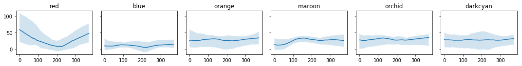
Predictions by climate
It would be cool to see why the model placed each station in each climate. These graphs are pretty cool, but I wouldn’t read too much into them!
I’ll group up weather stations by assigned climate, and ask the model to predict the weather every day of the year. Then for each day, I’ll plot the prediction of the median of all stations in that climate. To give an idea of the range of predictions in that climate, and shade in the area between the 5th and 95th percentile of stations.
In other words, on June 11, the precipitation chart will show a solid line where the median of the precipitation predictions for all stations. It shows a shaded region between the 5th and 95th percentile of precipitation predictions. (Note it’s not following a particular station! It’s just looking at all of the predictions for a day)
Temperature
It looks like blue (the West) and maroon (northern part of east of the Rockies) have colder winters.

Precipitation
I think the precipitation predictions look a little weird. That said, I approve that the red dots were mostly on the West Coast, and the precipitation predictions show that climate includes a lot of places with very rainy winters. And that blue, the West, includes more dry places.
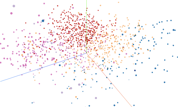
TensorBoard Projector
TensorBoard has a neat embedding visualization currently called Projector. If you add column headers to the tsv files the classifier outputs above, you can load them in as labels and kind of get an idea of what KMeans is doing!
Day of the year
This was funny: before I used the day of the year, I used separate values for the month and the year. Here is what the predictions looked like:
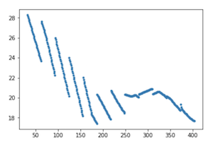 |
 |
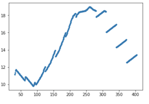 |
Basemap
I used Basemap to generate images. Here’s some of the code I used to generate the maps.
Inspiration
My sister told me about the problem with Köppen!
The neural network to learn embeddings is a little similar to how CBOW and Skip-Grams work.
What next?
This was a neat proof-of-concept! There are lots of directions one can take this project, but I’m out of time for today. A few off the top of my head are:
- Use more data!
- Snow data is often present in the dataset, so I don’t even need to deal with missing data.
- Try different representations of days, like using an embedding!
- Find a better way to choose the model.
[1] By Peel, M. C., Finlayson, B. L., and McMahon, T. A.(University of Melbourne)Enhanced, modified, and vectorized by Ali Zifan. - Hydrology and Earth System Sciences: “Updated world map of the Köppen-Geiger climate classification” (Supplement)map in PDF (Institute for Veterinary Public Health)Legend explanation, CC BY-SA 4.0, https://commons.wikimedia.org/w/index.php?curid=47086879
[2] Menne, M.J., I. Durre, R.S. Vose, B.E. Gleason, and T.G. Houston, 2012: An overview of the Global Historical Climatology Network-Daily Database. Journal of Atmospheric and Oceanic Technology, 29, 897-910, doi:10.1175/JTECH-D-11-00103.1.
[3] Menne, M.J., I. Durre, B. Korzeniewski, S. McNeal, K. Thomas, X. Yin, S. Anthony, R. Ray, R.S. Vose, B.E.Gleason, and T.G. Houston, 2012: Global Historical Climatology Network - Daily (GHCN-Daily), Version 3. NOAA National Climatic Data Center. http://doi.org/10.7289/V5D21VHZ 2018/06/09.