Bayesian linear regression with `pymc3`
In this post, I’ll revisit the Bayesian linear regression series, but use pymc3.
I’m still a little fuzzy on how pymc3 things work. Luckily it turns out that pymc3’s getting started tutorial includes this task.
Data generation
Data generation corresponds to Bayesian Linear Regression part 2: demo data (The order of the first two posts of the original series are interchangeable.)
I need to generate observed data to learn from. I’ll use the same model as before where the underlying function \( f \) is a line:
There’s Gaussian noise on the observations, so the observed values are
Like the pymc3 tutorial and my old posts, I’ll generate observed data with numpy:
N_points = 11

x = 2 * np.random.rand(N_points, 1) - 1

true_sigma_y = 0.1

def f(x):
    return 0.3 * x + 2

noise = true_sigma_y * np.random.randn(x.shape[0], 1)

Y = f(x) + noise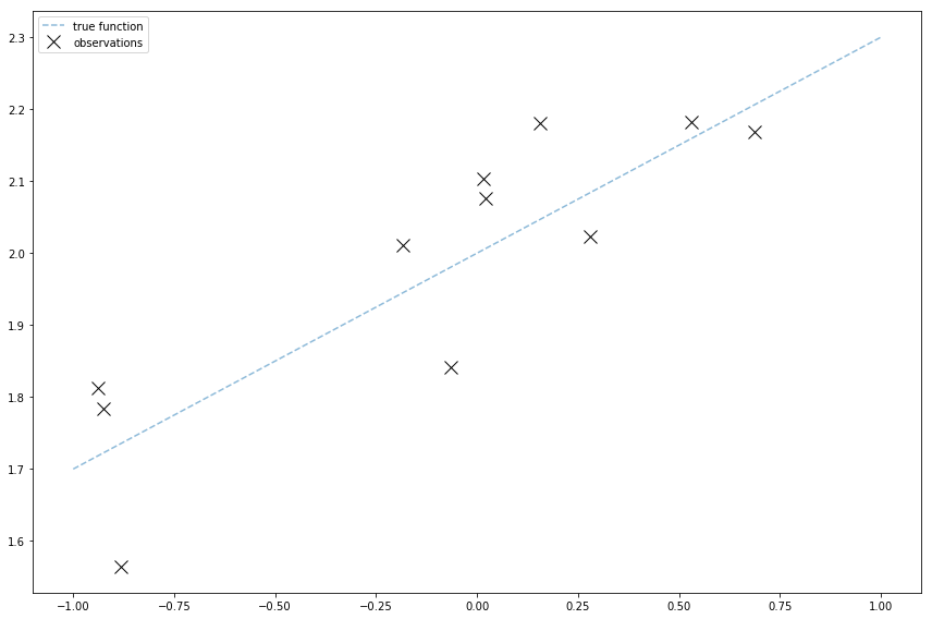
Sampling from the prior
This part corresponds to Bayesian Linear Regression part 1: plotting samples from the weight prior.
Now I’ll use pymc3! To sample from the weights prior, I need to set up my model. First I’ll copy over my hyperparameters from the old post.
(Note: I updated the subscript on the slope from _w to _m).
# weights on the priors
mu_m = 0
mu_b = 0

sigma_m = 0.2
sigma_b = 0.2
Before I sampled weights from the prior using:
w = np.random.randn(line_count, D) @ V_0 + w_0
Because \( V_0 \) is a diagonal matrix, this is like sampling from two single-variable Gaussians:
In pymc3, defining this model and sampling some weights from a model looks like:
mu_w = 0
mu_b = 0

sigma_w = 0.2
sigma_b = 0.2

model = pm.Model()

with model:
    m = pm.Normal('m', mu=mu_m, sd=sigma_m)
    b = pm.Normal('b', mu=mu_b, sd=sigma_b)

    prior_trace = pm.sample(200)
There are a few differences so far!
Importantly, by assuming the independence in the priors, pymc3 is going to learn a model that assumes \( w_b \) and \( w_m \) are independent. This is different than the original post, which also learned a covariance between the two weights.
Aside from the model set up, the action is already a little different! Before I was sampling from the normal distribution using np.random.randn, which can be done by sampling from a uniform distribution (a super common operation) and applying a transformation to it to scale it as a Gaussian.
pymc3 uses fancier sampling approaches (my last post on Gibbs sampling is another fancy sampling approach!) This is going to be a common theme in this post: The Gaussian linear regression model I’m using in these posts is a small Gaussian model, which is easy to work with and has a closed-form for its posterior. But this doesn’t work in complex models, so pymc3 uses approximate methods like fancy sampling instead. In other words, I’m using fancy things in pymc3 that are overkill for my particular model.
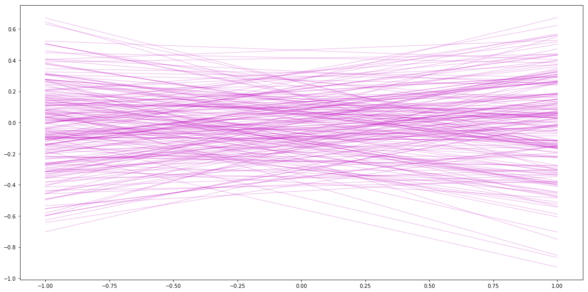
Visualizing
Next I can plot some of the slopes/intercepts sampled from the prior. It looks similar to the plots I got in my last post.
Sampling from the Posterior
This part corresponds to Bayesian Linear Regression part 3: Posterior and Bayesian Linear Regression part 4: Plots.
In the posterior post, I had a closed-form for the posterior of a Gaussian likelihood with a Gaussian prior.
In pymc3, I create a deterministic random variable exp_f that is \( f = mx + b \), where m and b are the random variables defined above, and x are the x-values for the observed data. I set that as the mean of a Normal distribution with the \( \sigma_y \) noise (and like the other posts assume I know the true noise sigma_y = true_sigma_y.) Then I can pass the observed values Y I came up with at the beginning. Then I sample again!
sigma_y = true_sigma_y
# Use the model defined above
with model:
exp_f = m * x + b
Y_obs = pm.Normal('Y_obs', mu=exp_f, sd=sigma_y, observed=Y)
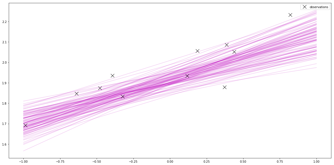
posterior_trace = pm.sample(200, tune=1000)Now I can plot a few of these. This is jumping ahead to “Sampling from the posterior” in Bayesian Linear Regression part 4: Plots. This is another interesting thing about pymc3 approaches.
Before, I used the closed-form of the mean and variance of the normal distribution that represents the posterior. Then I sampled from that distribution to plot samples from the posterior.
Using pymc3, I skip computing the posterior, and instead use clever methods to sample directly from the posterior. This is useful when the posterior is hard to compute.
pymc3 also gives me a cool plot of the samples.
pm.traceplot(posterior_trace)
Thoughts: Plotting error
That’s all I’m going to post for now. I wasn’t able to recreate all of the original series’ graphs using pymc3 yet.
One of my favorite graphs from the series was plotting a shaded area for the uncertainty from Bayesian Linear Regression part 4: Plots. There are two issues: in this post, I’m assuming the slope and intercept are independent, which is slightly different than that post, and I think that means the uncertainty is incorrectly clumped around 0 (because the form of the function that plots the uncertainty is based on \( ax^2 + 2bx + c \), where \( b \) is the covariance.) I started using pm.MvGaussian, which would find a covariance between the slope and intercept, but pm.summary(posterior_trace) gives me separate standard deviations for individual variables. I’ll post a follow-up if I can sort this out!