Using ipywidgets to learn machine learning

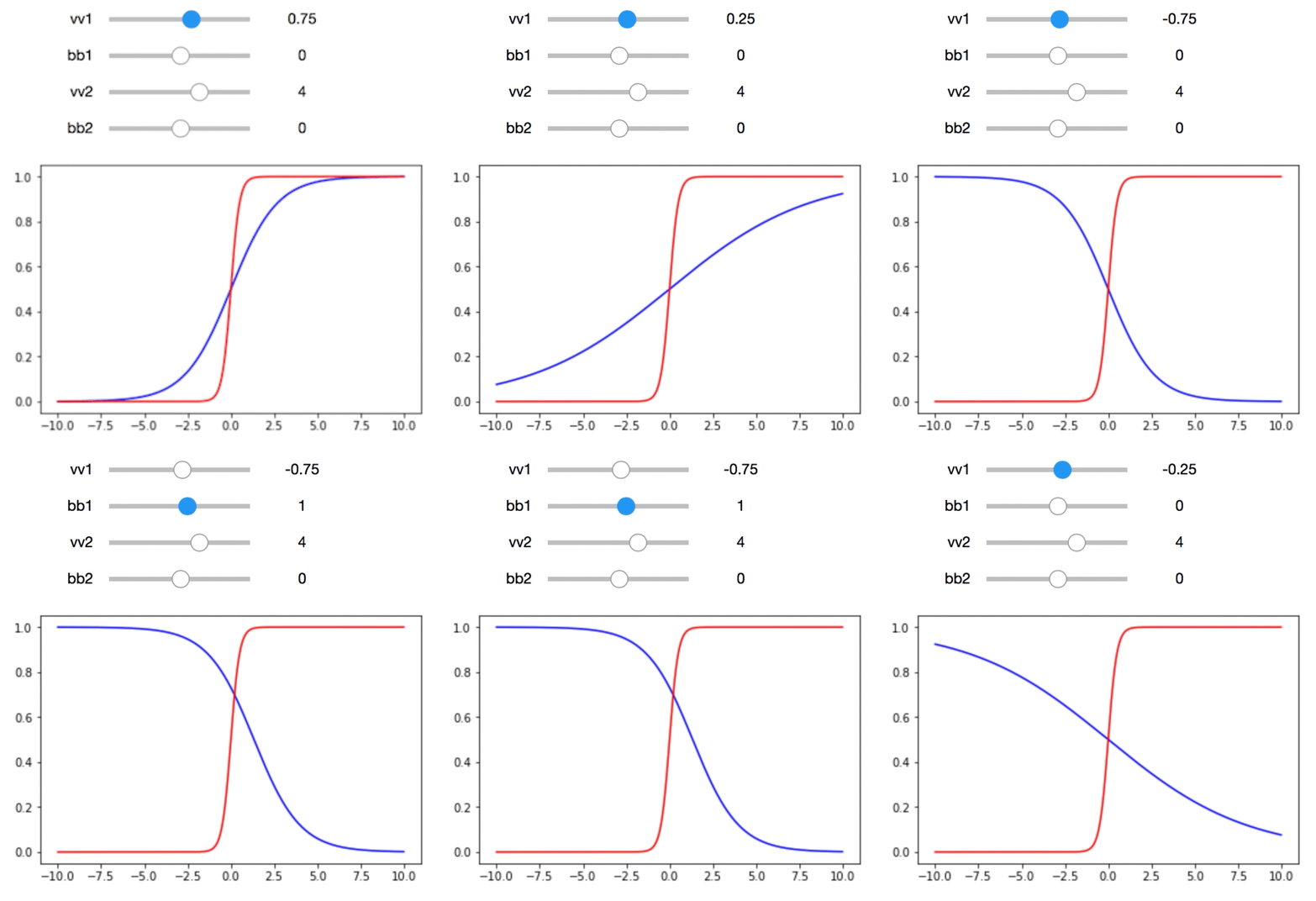
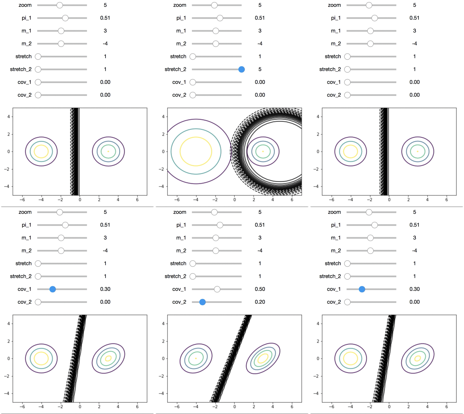
One of my favorite tricks in Jupyter notebooks is using ipywidgets.interact to explore an equation or dataset. Two equations I used it on were the logistic sigmoid and Bayes classifiers decision boundaries. (I also used ipywidgets to explore the dataset smallNORB.)

For example, to understand the logistic sigmoid function a little better, I used this:

which was created using:

import numpy as np
import matplotlib.pyplot as plt

from ipywidgets import interact

# The function I'm studying!
def logistic_sigmoid(xx, vv, b):
    return 1 / (1 + np.exp(-(np.dot(vv, xx) + b)))

plt.clf()
grid_size = 0.01
x_grid = np.arange(-5, 5, grid_size)


def plot_logistic_sigmoid(vv1, bb1, vv2, bb2):
    plt.plot(x_grid, logistic_sigmoid(x_grid, vv=vv1, b=bb1), '-b')
    plt.plot(x_grid, logistic_sigmoid(x_grid, vv=vv2, b=bb2), '-r')
    plt.axis([-5, 5, -0.5, 1.5])
    plt.show()


interact(
    plot_logistic_sigmoid,
    vv1=(-12, 10, .25),
    bb1=(-10, 10),
    vv2=(-10, 12),
    bb2=(-10, 10)
)

Bayes Classifiers with multivariate Gaussians

I did something similar for Bayes classifiers with multivariate Gaussians.